45 how to show data labels in excel

How To Show Or Hide Data Labels On MS Excel? - My ... 22 Dec 2019 — Select the chart on your MS Excel worksheet, A plus sign will appear at the top right corner of the table. · Now, you need to point to Data ... How to Add Labels to Show Totals in Stacked Column Charts in Excel In the chart, right-click the "Total" series and then, on the shortcut menu, select Add Data Labels. 9. Next, select the labels and then, in the Format Data Labels pane, under Label Options, set the Label Position to Above. 10. While the labels are still selected set their font to Bold. 11.

Custom Data Labels with Colors and Symbols in Excel Charts - [How To] Step 4: Select the data in column C and hit Ctrl+1 to invoke format cell dialogue box. From left click custom and have your cursor in the type field and follow these steps: Press and Hold ALT key on the keyboard and on the Numpad hit 3 and 0 keys. Let go the ALT key and you will see that upward arrow is inserted.

How to show data labels in excel

Excel - Axis Label Interval Option not available - Microsoft Community I can see no option available for me to specify the interval between axis labels in my excel chart. Please provide me with a solution as it will be beneficial to show data with specified interval labels, say 30 min intervals instead of 28 min intervals. I believe there is supposed to be an adjust intervals option in the labels section circled. How to add or move data labels in Excel chart? - ExtendOffice 1. Click the chart to show the Chart Elements button . 2. Then click the Chart Elements, and check Data Labels, then you can click the arrow to choose an option about the data labels in the sub menu. See screenshot: Custom Chart Data Labels In Excel With Formulas Follow the steps below to create the custom data labels. Select the chart label you want to change. In the formula-bar hit = (equals), select the cell reference containing your chart label's data. In this case, the first label is in cell E2. Finally, repeat for all your chart laebls.

How to show data labels in excel. Excel tutorial: How to use data labels Generally, the easiest way to show data labels to use the chart elements menu. When you check the box, you'll see data labels appear in the chart. If you have more than one data series, you can select a series first, then turn on data labels for that series only. You can even select a single bar, and show just one data label. Hiding data labels for some, not all values in a series - MrExcel Here's a good challenge for you. I can't figure it out, and I believe it's a limitation of Excel. I have a bar graph with several data series. I know how to show the data labels for every data point in a given series. But I'm looking to show the data label for only some data points in a given series -- i.e. non-zero valued data points. DataLabels.ShowValue property (Excel) | Microsoft Docs Example. This example enables the value to be shown for the data labels of the first series, on the first chart. This example assumes that a chart exists on the active worksheet. VB. Sub UseValue () ActiveSheet.ChartObjects (1).Activate ActiveChart.SeriesCollection (1) _ .DataLabels.ShowValue = True End Sub. how to add data labels into Excel graphs - storytelling with data 10 Feb 2021 — Right-click on a point and choose Add Data Label. You can choose any point to add a label—I'm strategically choosing the endpoint because that's ...

Excel Charts: Dynamic Label positioning of line series - XelPlus Go to Layout tab, select Data Labels > Right. Right mouse click on the data label displayed on the chart. Select Format Data Labels. Under the Label Options, show the Series Name and untick the Value. Show the Label Instead of the Value for Actual How to use data labels in a chart - YouTube Excel charts have a flexible system to display values called "data labels". Data labels are a classic example a "simple" Excel feature with a huge range of o... How to hide zero data labels in chart in Excel? - ExtendOffice In the Format Data Labelsdialog, Click Numberin left pane, then selectCustom from the Categorylist box, and type #""into the Format Codetext box, and click Addbutton to add it to Typelist box. See screenshot: 3. Click Closebutton to close the dialog. Then you can see all zero data labels are hidden. How do I add additional labels to an excel chart? - Stack Overflow I've got a chart in excel and I'd like to add additional labels to it. In the below example I want to add "Inadequate" next to the 34s, "Inconsistent" next to the 42 and so on. Ideally, I'd like to be able to tweek how the floating text looks. I've tried adding an extra row in my data below, but it just messes up the whole chart or isn't useful.

How to Change Excel Chart Data Labels to Custom Values? Now, click on any data label. This will select "all" data labels. Now click once again. At this point excel will select only one data label. Go to Formula bar, press = and point to the cell where the data label for that chart data point is defined. Repeat the process for all other data labels, one after another. See the screencast. Points to note: Change the format of data labels in a chart - Microsoft Support To get there, after adding your data labels, select the data label to format, and then click Chart Elements > Data Labels > More Options. To go to the appropriate area, click one of the four icons ( Fill & Line, Effects, Size & Properties ( Layout & Properties in Outlook or Word), or Label Options) shown here. How to Use Cell Values for Excel Chart Labels Select the chart, choose the "Chart Elements" option, click the "Data Labels" arrow, and then "More Options." Uncheck the "Value" box and check the "Value From Cells" box. Select cells C2:C6 to use for the data label range and then click the "OK" button. The values from these cells are now used for the chart data labels. Format Data Labels in Excel- Instructions - TeachUcomp, Inc. To do this, click the "Format" tab within the "Chart Tools" contextual tab in the Ribbon. Then select the data labels to format from the "Chart Elements" drop-down in the "Current Selection" button group. Then click the "Format Selection" button that appears below the drop-down menu in the same area.

Line Chart in Excel - Easy Excel Tutorial

Add a DATA LABEL to ONE POINT on a chart in Excel Click on the chart line to add the data point to. All the data points will be highlighted. Click again on the single point that you want to add a data label to. Right-click and select ' Add data label ' This is the key step! Right-click again on the data point itself (not the label) and select ' Format data label '.

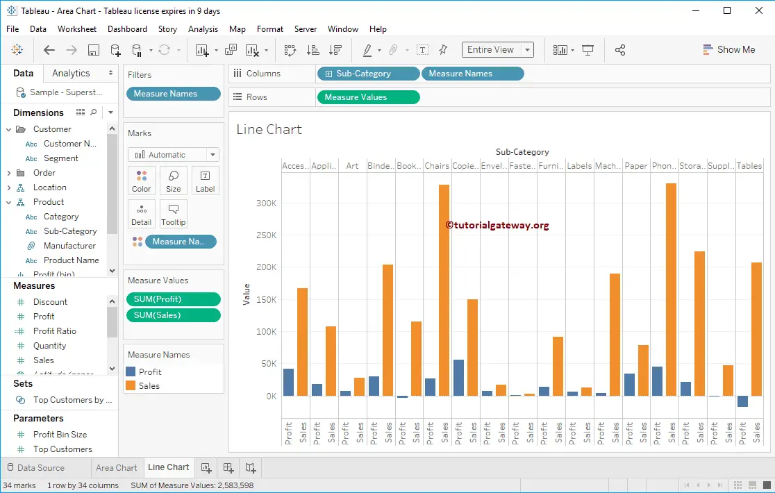
Grouped Bar Chart in Tableau

How to Add Data Labels in Excel - Excelchat | Excelchat In Excel 2013 and the later versions we need to do the followings; Click anywhere in the chart area to display the Chart Elements button Figure 5. Chart Elements Button Click the Chart Elements button > Select the Data Labels, then click the Arrow to choose the data labels position. Figure 6. How to Add Data Labels in Excel 2013 Figure 7.

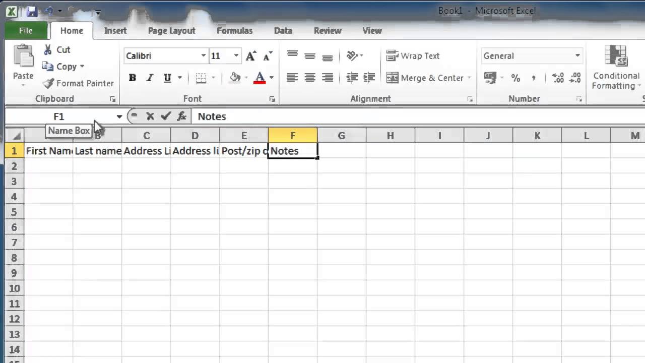
How to Make address book in Excel 2010 - YouTube

How to find, highlight and label a data point in Excel scatter plot Select the Data Labels box and choose where to position the label. By default, Excel shows one numeric value for the label, y value in our case. To display both x and y values, right-click the label, click Format Data Labels…, select the X Value and Y value boxes, and set the Separator of your choosing: Label the data point by name

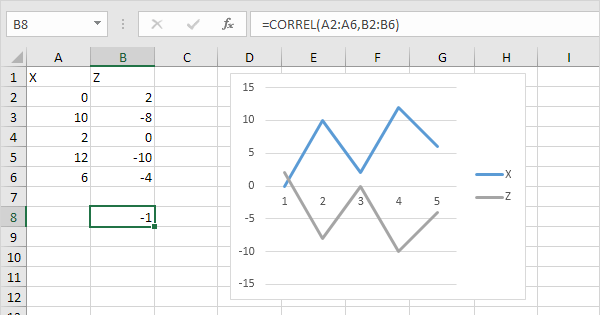
Correlation Analysis - Easy Excel Tutorial

How to Find, Highlight, and Label a Data Point in Excel Scatter Plot? By default, the data labels are the y-coordinates. Step 3: Right-click on any of the data labels. A drop-down appears. Click on the Format Data Labels… option. Step 4: Format Data Labels dialogue box appears. Under the Label Options, check the box Value from Cells . Step 5: Data Label Range dialogue-box appears.

MS Excel 2013: Display the fields in the Values Section in multiple ...

Excel charts: how to move data labels to legend You can't do that, but you can show a data table below the chart instead of data labels: Click anywhere on the chart. On the Design tab of the ribbon (under Chart Tools), in the Chart Layouts group, click Add Chart Element > Data Table > With Legend Keys (or No Legend Keys if you prefer)

Create a 3D Table Cube - YouTube

How to show data label in "percentage" instead of - Microsoft Community Select Format Data Labels Select Number in the left column Select Percentage in the popup options In the Format code field set the number of decimal places required and click Add. (Or if the table data in in percentage format then you can select Link to source.) Click OK Regards, OssieMac Report abuse 8 people found this reply helpful ·

Excel Charts: Positive/Negative Axis Labels on a Bar Chart

How to Add Data Labels to an Excel 2010 Chart - Dummies.com 26 Mar 2016 — Click anywhere on the chart that you want to modify. · On the Chart Tools Layout tab, click the Data Labels button in the Labels group. · Select ...

410 How to display percentage labels in pie chart in Excel 2016 - YouTube

Excel 2010: Show Data Labels In Chart - AddictiveTips With data labels, you can easily view the values that affects chart area in Excel 2010. Lets look at how to enable and use them. To enable data labels in chart, select the chart and head over to Chart Tools Layout tab, from Labels group, under Data Labels options, select a position. It will show Data labels at specified position.

Share :