44 add data labels to chart excel
Adding Data Labels To An Excel Chart | MyExcelOnline In our example below, I add a Data Label to a column chart and then I format the data label using CTRL+1. I then select to custom format the numbers so it shows the values as thousands by adding a comma , after each zero and then showing the work k by adding "k" Example Custom Number Format: [$$-1004]#,##0 ,"k" ;- [$$-1004]#,##0 ,"k" Adding rich data labels to charts in Excel 2013 | Microsoft 365 Blog To add a data label in a shape, select the data point of interest, then right-click it to pull up the context menu. Click Add Data Label, then click Add Data Callout . The result is that your data label will appear in a graphical callout. In this case, the category Thr for the particular data label is automatically added to the callout too.
How to Add Two Data Labels in Excel Chart (with Easy Steps) Step 4: Format Data Labels to Show Two Data Labels. Here, I will discuss a remarkable feature of Excel charts. You can easily show two parameters in the data label. For instance, you can show the number of units as well as categories in the data label. To do so, Select the data labels. Then right-click your mouse to bring the menu.

Add data labels to chart excel
How To Add Data Labels In Excel - danielsadventure.info Click on the arrow next to data labels to change the position of where the labels are in relation to the bar chart. Add A Label (Form Control) Click Developer, Click Insert, And Then Click Label. You can now configure the label as required — select the content of. To format data labels in excel, choose the set of data labels to format. Adding Data Labels to Your Chart (Microsoft Excel) To add data labels in Excel 2013 or later versions, follow these steps: Activate the chart by clicking on it, if necessary. Make sure the Design tab of the ribbon is displayed. (This will appear when the chart is selected.) Click the Add Chart Element drop-down list. Select the Data Labels tool. How to Add Data Labels in Excel - Excelchat | Excelchat After inserting a chart in Excel 2010 and earlier versions we need to do the followings to add data labels to the chart; Click inside the chart area to display the Chart Tools. Figure 2. Chart Tools Click on Layout tab of the Chart Tools. In Labels group, click on Data Labels and select the position to add labels to the chart. Figure 3.
Add data labels to chart excel. How to add Data Label to Waterfall chart - Excel Help Forum 1. Manually edit the text of the labels. 2. Select each label (two single clicks, one selects the series of labels, the second selects the individual label). Don't click so much as the cursor starts blinking in the label. Click in the formula bar, type an = sign, then click on the cell that contains the label. 3. How to create Custom Data Labels in Excel Charts - Efficiency 365 Create the chart as usual. Add default data labels. Click on each unwanted label (using slow double click) and delete it. Select each item where you want the custom label one at a time. Press F2 to move focus to the Formula editing box. Type the equal to sign. Now click on the cell which contains the appropriate label. Data Labels in Excel Pivot Chart (Detailed Analysis) Click on the Plus sign right next to the Chart, then from the Data labels, click on the More Options. After that, in the Format Data Labels, click on the Value From Cells. And click on the Select Range. In the next step, select the range of cells B5:B11. Click OK after this. Add / Move Data Labels in Charts - Excel & Google Sheets Adding Data Labels Click on the graph Select + Sign in the top right of the graph Check Data Labels Change Position of Data Labels Click on the arrow next to Data Labels to change the position of where the labels are in relation to the bar chart Final Graph with Data Labels
Custom Chart Data Labels In Excel With Formulas - How To Excel At Excel Follow the steps below to create the custom data labels. Select the chart label you want to change. In the formula-bar hit = (equals), select the cell reference containing your chart label's data. In this case, the first label is in cell E2. Finally, repeat for all your chart laebls. How to Add Data Labels to an Excel 2010 Chart - dummies Select where you want the data label to be placed. Data labels added to a chart with a placement of Outside End. On the Chart Tools Layout tab, click Data Labels→More Data Label Options. The Format Data Labels dialog box appears. How to Add Labels to Scatterplot Points in Excel - Statology Step 3: Add Labels to Points Next, click anywhere on the chart until a green plus (+) sign appears in the top right corner. Then click Data Labels, then click More Options… In the Format Data Labels window that appears on the right of the screen, uncheck the box next to Y Value and check the box next to Value From Cells. Excel charts: add title, customize chart axis, legend and data labels Click anywhere within your Excel chart, then click the Chart Elements button and check the Axis Titles box. If you want to display the title only for one axis, either horizontal or vertical, click the arrow next to Axis Titles and clear one of the boxes: Click the axis title box on the chart, and type the text.
Change the format of data labels in a chart To get there, after adding your data labels, select the data label to format, and then click Chart Elements > Data Labels > More Options. To go to the appropriate area, click one of the four icons ( Fill & Line, Effects, Size & Properties ( Layout & Properties in Outlook or Word), or Label Options) shown here. Add a DATA LABEL to ONE POINT on a chart in Excel Click on the chart line to add the data point to. All the data points will be highlighted. Click again on the single point that you want to add a data label to. Right-click and select ' Add data label ' This is the key step! Right-click again on the data point itself (not the label) and select ' Format data label '. Add data labels and callouts to charts in Excel 365 - EasyTweaks.com The steps that I will share in this guide apply to Excel 2021 / 2019 / 2016. Step #1: After generating the chart in Excel, right-click anywhere within the chart and select Add labels . Note that you can also select the very handy option of Adding data Callouts. How to add a line in Excel graph: average line, benchmark, etc. Right-click the selected data point and pick Add Data Label in the context menu: The label will appear at the end of the line giving more information to your chart viewers: Add a text label for the line. To improve your graph further, you may wish to add a text label to the line to indicate what it actually is. Here are the steps for this set up:
How-to Use Data Labels from a Range in an Excel Chart - Excel ...
How to add data labels in excel to graph or chart (Step-by-Step) Add data labels to a chart 1. Select a data series or a graph. After picking the series, click the data point you want to label. 2. Click Add Chart Element Chart Elements button > Data Labels in the upper right corner, close to the chart. 3. Click the arrow and select an option to modify the location. 4.

Display Customized Data Labels on Charts & Graphs
Add or remove data labels in a chart - support.microsoft.com Add data labels to a chart Click the data series or chart. To label one data point, after clicking the series, click that data point. In the upper right corner, next to the chart, click Add Chart Element > Data Labels. To change the location, click the arrow, and choose an option.

Add data labels and callouts to charts in Excel 365 ...
Adding Data Labels to Your Chart (Microsoft Excel) - ExcelTips (ribbon) To add data labels in Excel 2013 or later versions, follow these steps: Activate the chart by clicking on it, if necessary. Make sure the Design tab of the ribbon is displayed. (This will appear when the chart is selected.) Click the Add Chart Element drop-down list. Select the Data Labels tool.

Format Data Labels in Excel- Instructions - TeachUcomp, Inc.
Add Custom Labels to x-y Scatter plot in Excel Step 1: Select the Data, INSERT -> Recommended Charts -> Scatter chart (3 rd chart will be scatter chart) Let the plotted scatter chart be. Step 2: Click the + symbol and add data labels by clicking it as shown below. Step 3: Now we need to add the flavor names to the label. Now right click on the label and click format data labels.

How to add axis titles in excel chart | WPS Office Academy
How to Add Data Labels in Excel - Excelchat | Excelchat After inserting a chart in Excel 2010 and earlier versions we need to do the followings to add data labels to the chart; Click inside the chart area to display the Chart Tools. Figure 2. Chart Tools Click on Layout tab of the Chart Tools. In Labels group, click on Data Labels and select the position to add labels to the chart. Figure 3.

Adding rich data labels to charts in Excel 2013 | Microsoft ...
Adding Data Labels to Your Chart (Microsoft Excel) To add data labels in Excel 2013 or later versions, follow these steps: Activate the chart by clicking on it, if necessary. Make sure the Design tab of the ribbon is displayed. (This will appear when the chart is selected.) Click the Add Chart Element drop-down list. Select the Data Labels tool.

How-to Use Data Labels from a Range in an Excel Chart - Excel ...
How To Add Data Labels In Excel - danielsadventure.info Click on the arrow next to data labels to change the position of where the labels are in relation to the bar chart. Add A Label (Form Control) Click Developer, Click Insert, And Then Click Label. You can now configure the label as required — select the content of. To format data labels in excel, choose the set of data labels to format.

EXCEL Charts: Column, Bar, Pie and Line
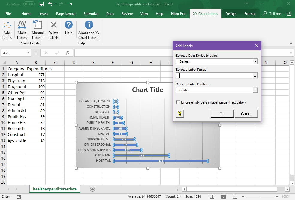
Add Labels to XY Chart Data Points in Excel with XY Chart Labeler
Excel tutorial: How to use data labels

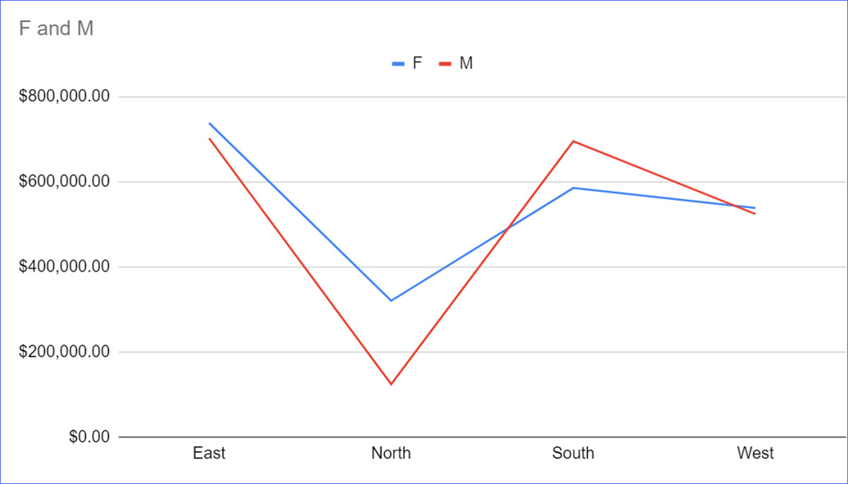
How to Place Labels Directly Through Your Line Graph in ...

How to Customize Your Excel Pivot Chart Data Labels - dummies

How to Add Data Labels to your Excel Chart in Excel 2013

How to add data labels from different column in an Excel chart?
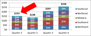
How to Add Totals to Stacked Charts for Readability - Excel ...

How to Add Data Labels to an Excel 2010 Chart - dummies

Adding rich data labels to charts in Excel 2013 | Microsoft ...
How to Add Data Labels to Charts in Google Sheets - ExcelNotes

How to add data labels from different column in an Excel chart?

how to add data labels into Excel graphs — storytelling with data

Adding rich data labels to charts in Excel 2013 | Microsoft ...

How to add or move data labels in Excel chart?
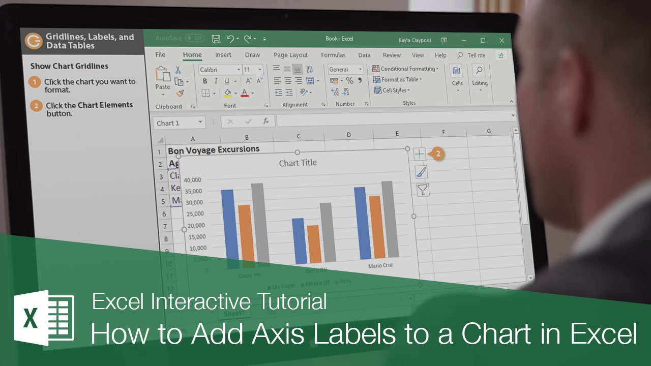
How to Add Axis Labels to a Chart in Excel | CustomGuide

Enable or Disable Excel Data Labels at the click of a button ...

Using the CONCAT function to create custom data labels for an ...

Change color of data label placed, using the 'best fit ...

Chart Data Labels in PowerPoint 2013 for Windows

charts - Excel, giving data labels to only the top/bottom X ...

How to Add Data Labels in Excel - Excelchat | Excelchat

Change the format of data labels in a chart

How to Make Pie Chart with Labels both Inside and Outside ...

How To Show Or Hide Data Labels On MS Excel? | My Windows Hub

Custom Data Labels with Colors and Symbols in Excel Charts ...

Add or remove data labels in a chart

Apply Custom Data Labels to Charted Points - Peltier Tech

How to add live total labels to graphs and charts in Excel ...

How to insert data labels to a Pie chart in Excel 2013

Adding rich data labels to charts in Excel 2013 | Microsoft ...

Microsoft Excel Tutorials: Add Data Labels to a Pie Chart

Apply Custom Data Labels to Charted Points - Peltier Tech
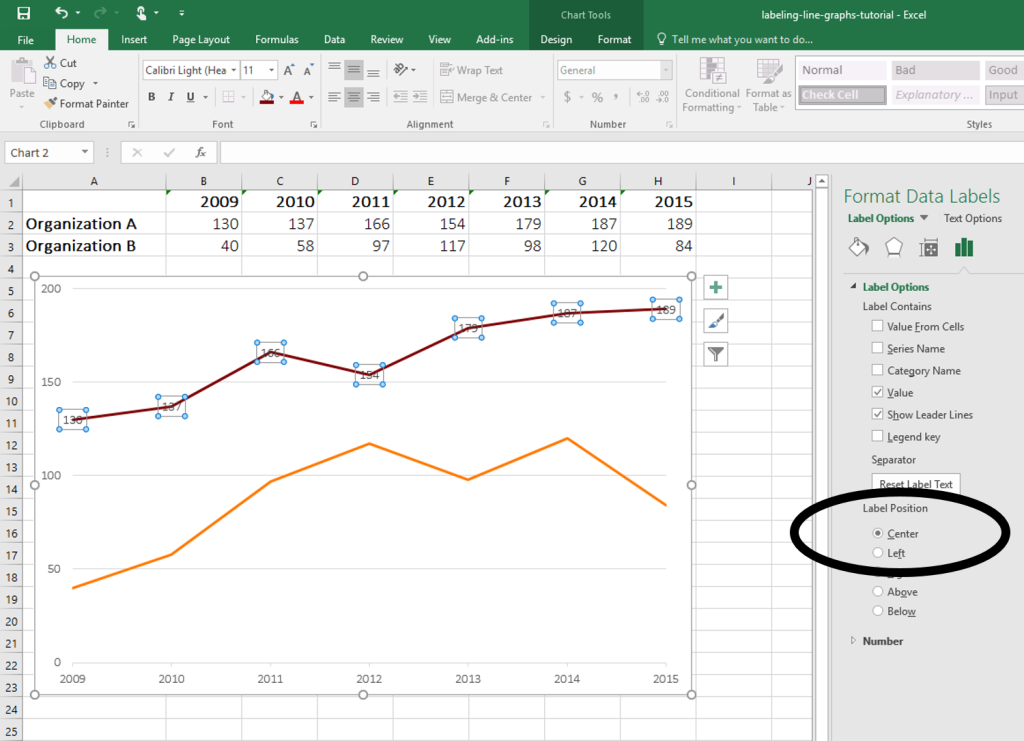
How to Place Labels Directly Through Your Line Graph in ...

Chart axes, legend, data labels, trendline in Excel - Tech Funda

424 How to add data label to line chart in Excel 2016

Improve your X Y Scatter Chart with custom data labels
Post a Comment for "44 add data labels to chart excel"