41 how to add axis labels in excel bar graph
How to add data labels from different column in an Excel chart? How to add total labels to stacked column chart in Excel? For stacked bar charts, you can add data labels to the individual components of the stacked bar chart easily. But this article will introduce solutions to add a floating total values displayed at the top of a stacked bar graph so that make the chart more understandable and readable. How to group (two-level) axis labels in a chart in Excel? - ExtendOffice (1) In Excel 2007 and 2010, clicking the PivotTable > PivotChart in the Tables group on the Insert Tab; (2) In Excel 2013, clicking the Pivot Chart > Pivot Chart in the Charts group on the Insert tab. 2. In the opening dialog box, check the Existing worksheet option, and then select a cell in current worksheet, and click the OK button. 3.
HOW TO CREATE A BAR CHART WITH LABELS INSIDE BARS IN EXCEL - simplexCT 7. In the chart, right-click the Series "# Footballers" Data Labels and then, on the short-cut menu, click Format Data Labels. 8. In the Format Data Labels pane, under Label Options selected, set the Label Position to Inside End. 9. Next, in the chart, select the Series 2 Data Labels and then set the Label Position to Inside Base.

How to add axis labels in excel bar graph
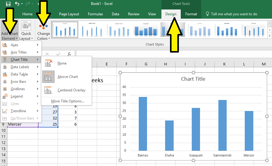
Bar Chart In Excel - How to Make/Create Bar Graph? (Examples) The steps to add Bar graph in Excel are as follows: Step 1: Select the data to create a Bar Chart. Step 2: Go to the Insert tab. Step 3: Select the Insert Column or Bar Chart option from the Charts group. Step 4: Choose the desired bar chart type we want from the drop-down list. Step 5: The Chart Design tab appears. Change axis labels in a chart in Office - support.microsoft.com In charts, axis labels are shown below the horizontal (also known as category) axis, next to the vertical (also known as value) axis, and, in a 3-D chart, next to the depth axis. The chart uses text from your source data for axis labels. To change the label, you can change the text in the source data. › documents › excelHow to add data labels from different column in an Excel chart? This method will introduce a solution to add all data labels from a different column in an Excel chart at the same time. Please do as follows: 1. Right click the data series in the chart, and select Add Data Labels > Add Data Labels from the context menu to add data labels. 2.
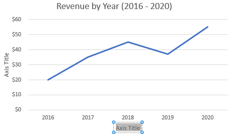
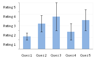
How to add axis labels in excel bar graph. Text Labels on a Horizontal Bar Chart in Excel - Peltier Tech On the Excel 2007 Chart Tools > Layout tab, click Axes, then Secondary Horizontal Axis, then Show Left to Right Axis. Now the chart has four axes. We want the Rating labels at the bottom of the chart, and we'll place the numerical axis at the top before we hide it. In turn, select the left and right vertical axes. How to Insert Axis Labels In An Excel Chart | Excelchat We will go to Chart Design and select Add Chart Element Figure 6 - Insert axis labels in Excel In the drop-down menu, we will click on Axis Titles, and subsequently, select Primary vertical Figure 7 - Edit vertical axis labels in Excel Now, we can enter the name we want for the primary vertical axis label. How To Add Axis Labels In Excel - BSUPERIOR Add Title one of your chart axes according to Method 1 or Method 2. Select the Axis Title. (picture 6) Picture 4- Select the axis title Click in the Formula Bar and enter =. Select the cell that shows the axis label. (in this example we select X-axis) Press Enter. Picture 5- Link the chart axis name to the text excel.officetuts.net › examples › add-percentageHow to Add Percentage Axis to Chart in Excel Add Percentage Axis to Chart as Secondary. The above is a fairly easy example as we had only percentages to deal with. Now we want to present all of the data we have on one chart. Luckily, newer versions of Excel are pretty helpful in this regard. We will select our table and then go to Insert >> Charts >> Recommended Charts:
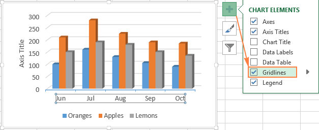
How to add axis label to chart in Excel? - ExtendOffice You can insert the horizontal axis label by clicking Primary Horizontal Axis Title under the Axis Title drop down, then click Title Below Axis, and a text box will appear at the bottom of the chart, then you can edit and input your title as following screenshots shown. 4. Legends in Chart | How To Add and Remove Legends In Excel … This has been a guide to Legend in Chart. Here we discuss how to add, remove and change the position of legends in an Excel chart, along with practical examples and a downloadable excel template. You can also go through our other suggested articles – Line Chart in Excel; Excel Bar Chart; Pie Chart in Excel; Scatter Chart in Excel How to Make a Bar Chart in Microsoft Excel - How-To Geek To add axis labels to your bar chart, select your chart and click the green "Chart Elements" icon (the "+" icon). From the "Chart Elements" menu, enable the "Axis Titles" checkbox. Axis labels should appear for both the x axis (at the bottom) and the y axis (on the left). These will appear as text boxes. peltiertech.com › broken-y-axis-inBroken Y Axis in an Excel Chart - Peltier Tech Nov 18, 2011 · On Microsoft Excel 2007, I have added a 2nd y-axis. I want a few data points to share the data for the x-axis but display different y-axis data. When I add a second y-axis these few data points get thrown into a spot where they don’t display the x-axis data any longer! I have checked and messed around with it and all the data is correct.
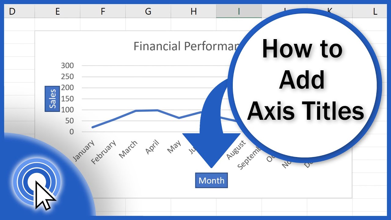
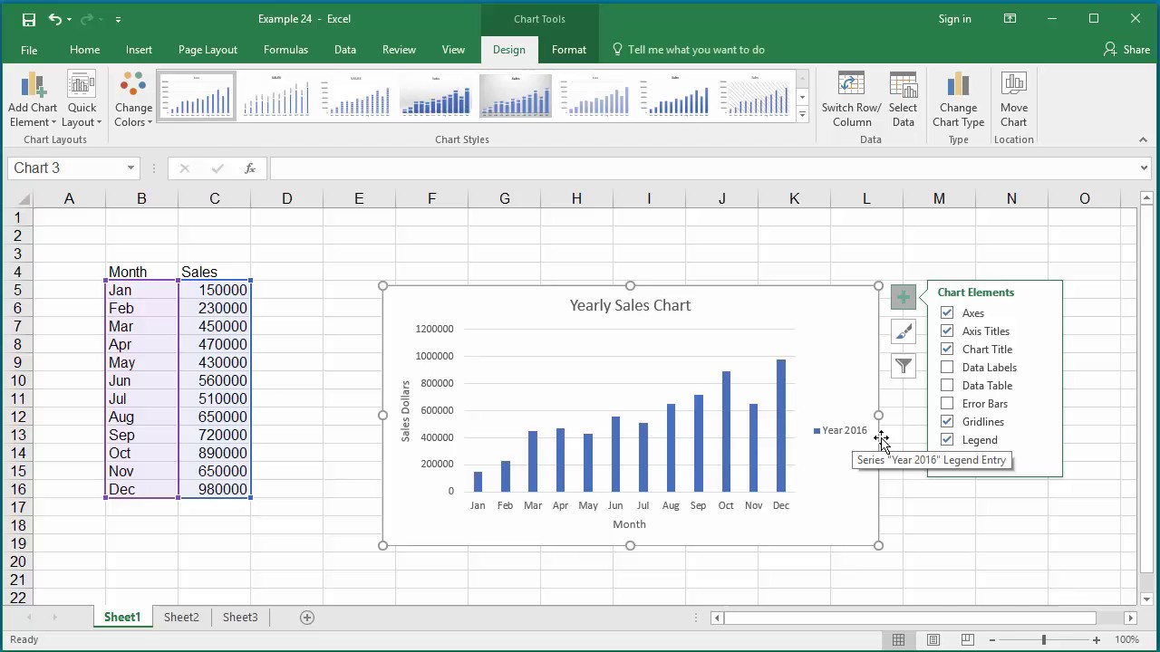
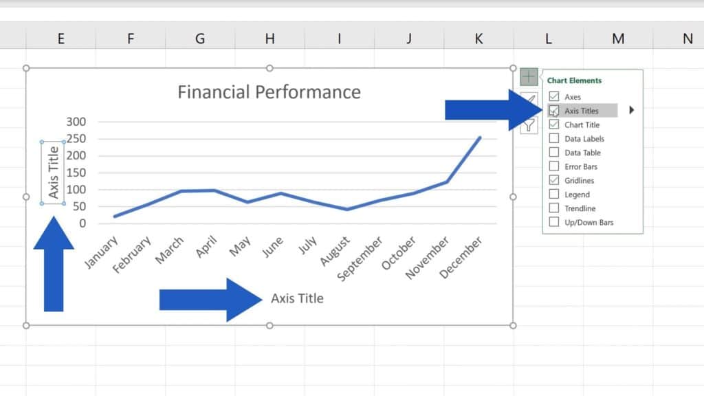
How to Add Axis Labels in Excel Charts - Step-by-Step (2022) - Spreadsheeto How to add axis titles 1. Left-click the Excel chart. 2. Click the plus button in the upper right corner of the chart. 3. Click Axis Titles to put a checkmark in the axis title checkbox. This will display axis titles. 4. Click the added axis title text box to write your axis label. How to add a total to a stacked column or bar chart in PowerPoint or Excel 07.09.2017 · Add data labels to the total segment at the Inside Base position so they are at the far left side of the segment. Using the default horizontal axis you will notice that there is a lot of blank ... Mar 26, 2016 - olrv.hoanglongcms.info By default, Excel writes the text string "Chart. This is done by editing the Horizontal (Category) axis labels. Click on the Edit button to add task names to the Horizontal (Category) axis labels. 3. Format the chart to make it look like a Gantt Chart. The stacked bar is ready. Your tasks are laid out on the chart as blue and orange bars. Custom Axis Labels and Gridlines in an Excel Chart The labels are (temporarily) shaded yellow to distinguish them from the built-in axis labels. Select the horizontal dummy series and add data labels. In Excel 2007-2010, go to the Chart Tools > Layout tab > Data Labels > More Data Label Options. In Excel 2013, click the "+" icon to the top right of the chart, click the right arrow next to ...
Add horizontal axis labels - VBA Excel - Stack Overflow
How do I add axis labels to bar chart bars? [SOLVED] For a new thread (1st post), scroll to Manage Attachments, otherwise scroll down to GO ADVANCED, click, and then scroll down to MANAGE ATTACHMENTS and click again. Now follow the instructions at the top of that screen. New Notice for experts and gurus:
How to Add Axis Titles in Excel
› charts › axis-textChart Axis – Use Text Instead of Numbers - Automate Excel Change Labels. While clicking the new series, select the + Sign in the top right of the graph; Select Data Labels; Click on Arrow and click Left . 4. Double click on each Y Axis line type = in the formula bar and select the cell to reference . 5. Click on the Series and Change the Fill and outline to No Fill . 6.

EXCEL Charts: Column, Bar, Pie and Line
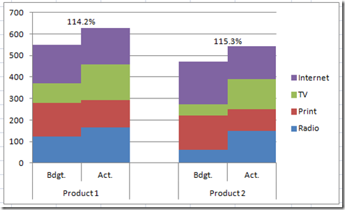
› pulse › how-add-total-stackedHow to add a total to a stacked column or bar chart in ... Sep 07, 2017 · The method used to add the totals to the top of each column is to add an extra data series with the totals as the values. Change the graph type of this series to a line graph.
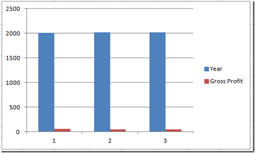
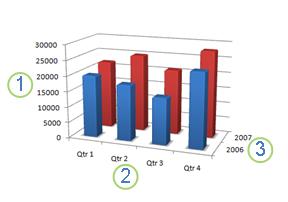
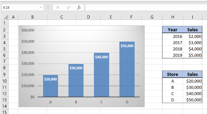
How-to Make Excel Put Years as the Chart Horizontal Axis ...
› excel › how-to-add-total-dataHow to Add Total Data Labels to the Excel Stacked Bar Chart Apr 03, 2013 · Step 4: Right click your new line chart and select “Add Data Labels” Step 5: Right click your new data labels and format them so that their label position is “Above”; also make the labels bold and increase the font size. Step 6: Right click the line, select “Format Data Series”; in the Line Color menu, select “No line”
Excel charts: add title, customize chart axis, legend and ...
Broken Y Axis in an Excel Chart - Peltier Tech 18.11.2011 · On Microsoft Excel 2007, I have added a 2nd y-axis. I want a few data points to share the data for the x-axis but display different y-axis data. When I add a second y-axis these few data points get thrown into a spot where they don’t display the x-axis data any longer! I have checked and messed around with it and all the data is correct. Can ...

How to Add Axis Titles in a Microsoft Excel Chart
How to add a line in Excel graph: average line, benchmark, etc. Copy the average/benchmark/target value in the new rows and leave the cells in the first two columns empty, as shown in the screenshot below. Select the whole table with the empty cells and insert a Column - Line chart. Now, our graph clearly shows how far the first and last bars are from the average: That's how you add a line in Excel graph.
How-to Add Centered Labels Above an Excel Clustered Stacked ...
Excel tutorial: How to customize axis labels Instead you'll need to open up the Select Data window. Here you'll see the horizontal axis labels listed on the right. Click the edit button to access the label range. It's not obvious, but you can type arbitrary labels separated with commas in this field. So I can just enter A through F. When I click OK, the chart is updated.
How to Change Horizontal Axis Labels in Excel 2010 - Solve ...
How to Add Axis Labels in Microsoft Excel - Appuals.com Click anywhere on the chart you want to add axis labels to. Click on the Chart Elements button (represented by a green + sign) next to the upper-right corner of the selected chart. Enable Axis Titles by checking the checkbox located directly beside the Axis Titles option. Once you do so, Excel will add labels for the primary horizontal and ...

How to label x and y axis in Microsoft excel 2016
How to Add Axis Labels to a Chart in Excel | CustomGuide Select the set of gridlines you want to show. Add Data Labels Use data labels to label the values of individual chart elements. Select the chart. Click the Chart Elements button. Click the Data Labels check box. In the Chart Elements menu, click the Data Labels list arrow to change the position of the data labels. Display a Data Table
How to Change Elements of a Chart like Title, Axis Titles, Legend etc in Excel 2016
How to format axis labels individually in Excel - SpreadsheetWeb Double-click on the axis you want to format. Double-clicking opens the right panel where you can format your axis. Open the Axis Options section if it isn't active. You can find the number formatting selection under Number section. Select Custom item in the Category list. Type your code into the Format Code box and click Add button.

Excel charts: add title, customize chart axis, legend and ...
How to Add Percentage Axis to Chart in Excel We will get a window on the right side of our screen with Axis options shown. We will click on the Numbers, then choose Percentage under Category: Our Chart now looks like this: Add Percentage Axis to Chart as Secondary. The above is a fairly easy example as we had only percentages to deal with. Now we want to present all of the data we have on ...
Graphing with Excel - BIOLOGY FOR LIFE
HOW TO CREATE A BAR CHART WITH LABELS ABOVE BAR IN EXCEL - simplexCT In the chart, right-click the Series "Dummy" Data Labels and then, on the short-cut menu, click Format Data Labels. 15. In the Format Data Labels pane, under Label Options selected, set the Label Position to Inside End. 16. Next, while the labels are still selected, click on Text Options, and then click on the Textbox icon. 17.
How to add Axis Labels (X & Y) in Excel & Google Sheets ...
How to Add a Secondary Axis in Excel Charts (Easy Guide) Below are the steps to add a secondary axis to the chart manually: Select the data set Click the Insert tab. In the Charts group, click on the Insert Columns or Bar chart option. Click the Clustered Column option. In the resulting chart, select the profit margin bars.

Excel charts: add title, customize chart axis, legend and ...
10 Design Tips to Create Beautiful Excel Charts and Graphs in … 24.09.2015 · 3) Shorten Y-axis labels. Long Y-axis labels, like large number values, take up a lot of space and can look a little messy, like in the chart below: To shorten them, right-click one of the labels on the Y-axis and choose "Format Axis" from the menu that appears. Choose "Number" from the lefthand side, then "Custom" from the Category list.
Change the display of chart axes
Skip Dates in Excel Chart Axis - My Online Training Hub 28.01.2015 · Excel Add-ins; Excel Forum. Register as Forum Member; Cart; Login; Skip Dates in Excel Chart Axis . January 28, 2015 by Mynda Treacy. In this tutorial we're going to look at how we can skip dates in the Excel chart axis for those dates that have no data. When you plot data in a chart that has a time axis Excel is clever enough to recognise you’re using dates and …

How to group (two-level) axis labels in a chart in Excel?
How to add Axis Labels (X & Y) in Excel & Google Sheets Adding Axis Labels Double Click on your Axis Select Charts & Axis Titles 3. Click on the Axis Title you want to Change (Horizontal or Vertical Axis) 4. Type in your Title Name Axis Labels Provide Clarity Once you change the title for both axes, the user will now better understand the graph.
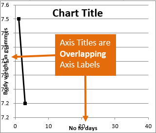
Resize the Plot Area in Excel Chart - Titles and Labels Overlap
Change axis labels in a chart - support.microsoft.com Right-click the category labels you want to change, and click Select Data. In the Horizontal (Category) Axis Labels box, click Edit. In the Axis label range box, enter the labels you want to use, separated by commas. For example, type Quarter 1,Quarter 2,Quarter 3,Quarter 4. Change the format of text and numbers in labels
EXCEL Charts: Column, Bar, Pie and Line
Excel charts: add title, customize chart axis, legend and data labels If you want to display the title only for one axis, either horizontal or vertical, click the arrow next to Axis Titles and clear one of the boxes: Click the axis title box on the chart, and type the text. To format the axis title, right-click it and select Format Axis Title from the context menu.

Change axis labels in a chart
How to Add X and Y Axis Labels in Excel (2 Easy Methods) Then go to Add Chart Element and press on the Axis Titles. Moreover, select Primary Horizontal to label the horizontal axis. In short: Select graph > Chart Design > Add Chart Element > Axis Titles > Primary Horizontal. Afterward, if you have followed all steps properly, then the Axis Title option will come under the horizontal line.

Moving the axis labels when a PowerPoint chart/graph has both ...
Chart Axis - Use Text Instead of Numbers - Automate Excel Change Labels. While clicking the new series, select the + Sign in the top right of the graph; Select Data Labels; Click on Arrow and click Left . 4. Double click on each Y Axis line type = in the formula bar and select the cell to reference . 5. Click on the Series and Change the Fill and outline to No Fill . 6.
How to Add Axis Titles in Excel
How to Label Axes in Excel: 6 Steps (with Pictures) - wikiHow Select the graph. Click your graph to select it. 3 Click +. It's to the right of the top-right corner of the graph. This will open a drop-down menu. 4 Click the Axis Titles checkbox. It's near the top of the drop-down menu. Doing so checks the Axis Titles box and places text boxes next to the vertical axis and below the horizontal axis.
Help Online - Quick Help - FAQ-154 How do I customize the ...
How to Show Percentage in Bar Chart in Excel (3 Handy Methods) - ExcelDemy 📌 Step 02: Insert Stacked Column Chart and Add Labels Secondly, select the dataset and navigate to Insert > Insert Column or Bar Chart > Stacked Column Chart. Similar to the previous method, switch the rows and columns and choose the Years as the x-axis labels. Next, go to Chart Element > Data Labels.

How to Add Axis Titles in a Microsoft Excel Chart
How to Add Total Data Labels to the Excel Stacked Bar Chart 03.04.2013 · Step 4: Right click your new line chart and select “Add Data Labels” Step 5: Right click your new data labels and format them so that their label position is “Above”; also make the labels bold and increase the font size. Step 6: Right click the line, select “Format Data Series”; in the Line Color menu, select “No line”

In an Excel chart, how do you craft X-axis labels with whole ...
› how-to-make-a-3-axis-graphHow to make a 3 Axis Graph using Excel? - GeeksforGeeks Jun 20, 2022 · In this article, we will learn how to create a three-axis graph in excel. Creating a 3 axis graph. By default, excel can make at most two axis in the graph. There is no way to make a three-axis graph in excel. The three axis graph which we will make is by generating a fake third axis from another graph. Given a data set, of date and ...

How to Add Axis Labels in Excel Charts - Step-by-Step (2022)
How to Add Axis Titles in a Microsoft Excel Chart - How-To Geek Select the chart and go to the Chart Design tab. Click the Add Chart Element drop-down arrow, move your cursor to Axis Titles, and deselect "Primary Horizontal," "Primary Vertical," or both. In Excel on Windows, you can also click the Chart Elements icon and uncheck the box for Axis Titles to remove them both.
Change the display of chart axes
How to make a 3 Axis Graph using Excel? - GeeksforGeeks 20.06.2022 · In this article, we will learn how to create a three-axis graph in excel. Creating a 3 axis graph. By default, excel can make at most two axis in the graph. There is no way to make a three-axis graph in excel. The three axis graph which we will make is by generating a fake third axis from another graph. Given a data set, of date and ...

How to add live total labels to graphs and charts in Excel ...
› documents › excelHow to add data labels from different column in an Excel chart? This method will introduce a solution to add all data labels from a different column in an Excel chart at the same time. Please do as follows: 1. Right click the data series in the chart, and select Add Data Labels > Add Data Labels from the context menu to add data labels. 2.
Adding chart title and axis-titles - YouTube
Change axis labels in a chart in Office - support.microsoft.com In charts, axis labels are shown below the horizontal (also known as category) axis, next to the vertical (also known as value) axis, and, in a 3-D chart, next to the depth axis. The chart uses text from your source data for axis labels. To change the label, you can change the text in the source data.
ggplot2 - Multirow axis labels with nested grouping variables ...
Bar Chart In Excel - How to Make/Create Bar Graph? (Examples) The steps to add Bar graph in Excel are as follows: Step 1: Select the data to create a Bar Chart. Step 2: Go to the Insert tab. Step 3: Select the Insert Column or Bar Chart option from the Charts group. Step 4: Choose the desired bar chart type we want from the drop-down list. Step 5: The Chart Design tab appears.

How-to Highlight Specific Horizontal Axis Labels in Excel ...
Text Labels on a Vertical Column Chart in Excel - Peltier Tech

How to add axis label to chart in Excel?
Excel Chart Axis Label Tricks • My Online Training Hub

How To Add Axis Labels In Excel - BSUPERIOR

Add or remove titles in a chart
How to Change Axis Values in Excel | Excelchat
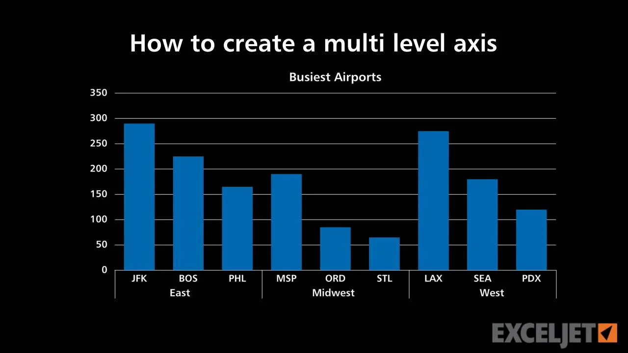
How to create a multi level axis

How to Add Axis Labels to a Chart in Excel | CustomGuide

Excel charts: add title, customize chart axis, legend and ...

How to Label Axes in Excel: 6 Steps (with Pictures) - wikiHow

Rule 24: Label your bars and axes — AddTwo
Post a Comment for "41 how to add axis labels in excel bar graph"