42 pivot table 2 row labels
› Add-a-Field-to-a-Pivot-TableHow to Add a Field to a Pivot Table: 14 Steps (with Pictures) Mar 28, 2019 · Adding a field to a pivot table gives you another way to refine, sort and filter the data. The field you choose to add to your pivot table can be used as a row label, column label or even a report filter, depending upon your needs. Regardless of the scenario, we've got you covered. Excel basics Resources or tips : r/excel - reddit.com chart properties (title, data range, data labels, legend, trendline), modify a chart, sparklines Other: Check spelling, absolute refencing, defined names, and print preview I wanted to know if you guys know any tips or resources I can use to make sure im prepped for the exam.
LOOKUPVALUE - DAX Guide -- LOOKUPVALUE searches in a table for the value of a column in a row -- that satisfy a set of equality conditions EVALUATE VAR SampleCustomers = SAMPLE ( 10, Customer, Customer[Customer Code] ) RETURN ADDCOLUMNS ( SUMMARIZE ( SampleCustomers, Customer[Customer Name], Customer[Birth Date] ), "Day of week on birthday in 2009", VAR BirthDate = Customer[Birth Date] VAR ReferenceYear = 2009 VAR ...
Pivot table 2 row labels
Ignore blank value in Pivot table Row labels with Apache POI Ignore blank value in Pivot table Row labels with Apache POI. I am trying to remove the blank row tables from the Pivot table. I couldn't find the documentation with Apache POI around it. Is there anybody achieved this or knows whether Apache POI supports this or not? How to Get Data from Another Sheet Based on Cell Value in Excel - ExcelDemy 1. Combining INDEX and MATCH Functions. Our first method is based on using the combination of INDEX and MATCH functions to get data from another sheet based on the cell value in Excel. The MATCH function in Excel is used to locate the position of a lookup value in a row, column, or table. The INDEX function returns a value or reference of the ... How to Build Excel UserForm With Dependent ComboBoxes Lists See the UserForm. To see the data entry UserForm: In Excel, press Alt+F11. In the Project Explorer, find the PartLocDbComboRibbonDepend file. Click the plus sign at the left of the Forms folder. Double-click the frmParts UserForm, to show it in the Code window.
Pivot table 2 row labels. CONCATENATEX - DAX Guide This article describes how to correctly use column references when manipulating tables assigned to DAX variables, avoiding syntax errors and making the code easier to read and maintain. » Read more. This article showcases the use of CONCATENATEX, a handy DAX function to return a list of values in a measure. How to insert a blank column in pivot table? - Chandoo.org 16/04/2015 · We all know pivot table functionality is a powerful & useful feature. But it comes with some quirks. For example, we cant insert a blank row or column inside pivot tables. So today let me share a few ideas on how you can insert a blank column. But first let's try inserting a column Imagine you are looking at a pivot table like above. And you want to insert a column or row. … Pivot To Rows Convert Columns [WJA6NU] we will see these features in details in this post group by convert (varchar,saledate,103) pivot basic syntax: select [non-pivoted column], first pivoted column as [column name], second pivoted column as [column name], last pivoted column as [column name] from ( [select query that produces the data]) as [alias for the source query] pivot ( … support.google.com › datastudio › answerPivot table reference - Data Studio Help - Google Example pivot table showing revenue per user, by country, quarter, and year. This table easily summarizes the data from the previous example. You can also quickly spot outliers or anomalies in your data. Notice that several countries had no revenue in Q4, for example. Pivot tables in Data Studio support adding multiple row and column dimensions.
How to Create a Report in Excel - Lifewire Select Insert > PivotTable . In the Create PivotTable dialogue, in the Table/Range field, select the range of data you want to analyze. In the Location field, select the first cell of the worksheet where you want the analysis to go. Select OK to finish. This will launch the pivot table creation process in the new sheet. › excel-pivot-table-formatHow to Format Excel Pivot Table - Contextures Excel Tips Jun 22, 2022 · Video: Change Pivot Table Labels. Watch this short video tutorial to see how to make these changes to the pivot table headings and labels. Get the Sample File. No Macros: To experiment with pivot table styles and formatting, download the sample file. The zipped file is in xlsx format, and and does NOT contain any macros. Export data from a Power BI visualization - Power BI For a matrix visual, each row can have 1 or more data intersections, so the exported rows count can be less than 150,000. (For example, if a matrix visual has 3 data intersections per row, the maximum row count will be 150,000 / 3 = 50,000 rows.) The message " Exported data exceeded the allowed volume. Formatting issues pls help..Is there a way to format Individual Measure ... It will create a separate legend for each measure. Then you are going to clic on the Show labels button in the toolbar: In this case, you will have a highlight table. Next, your format tips. When you want a white row, you format the legend with the start value as same as the end value, divergent pallete and color white.
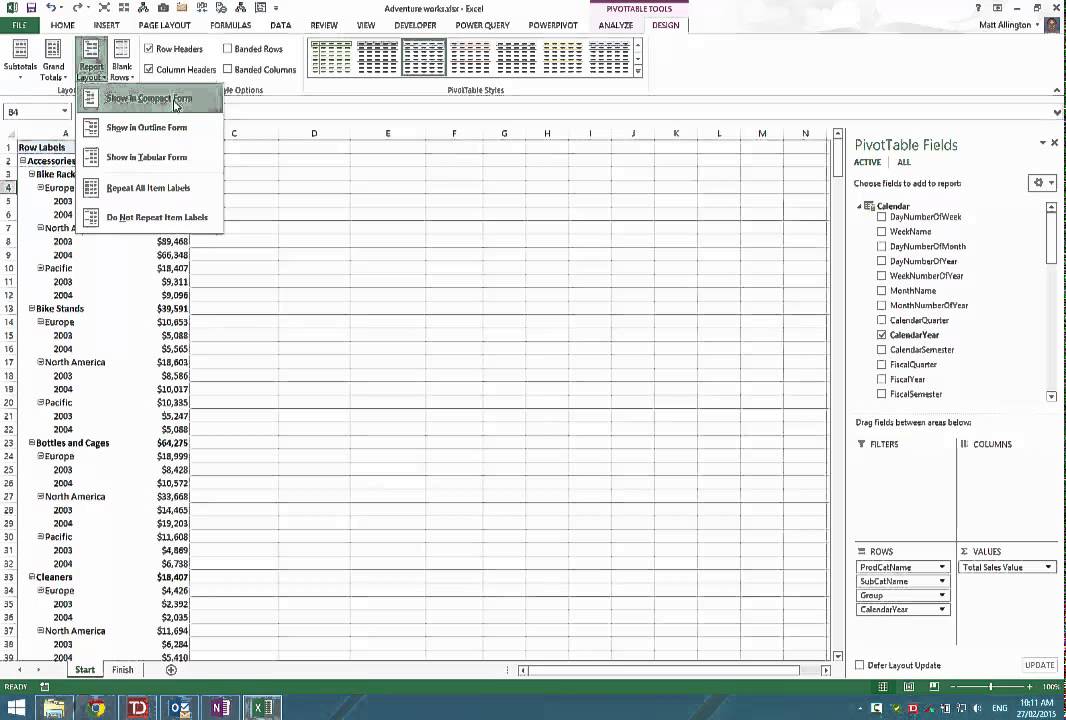
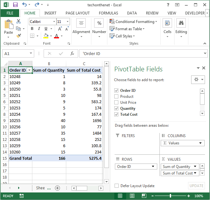
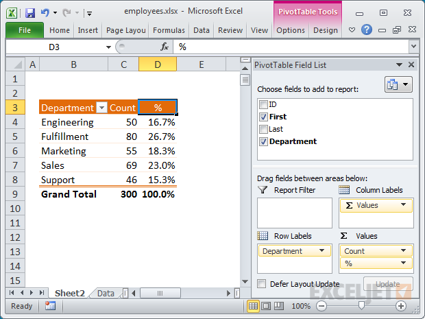
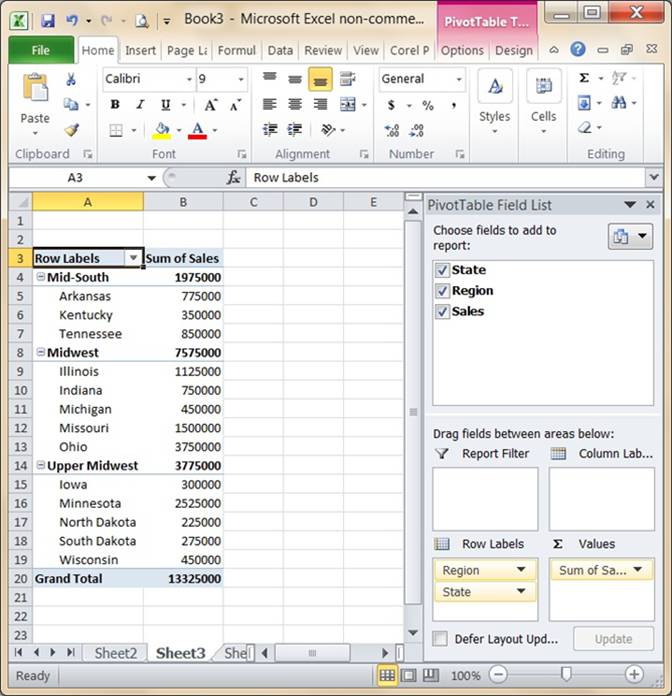
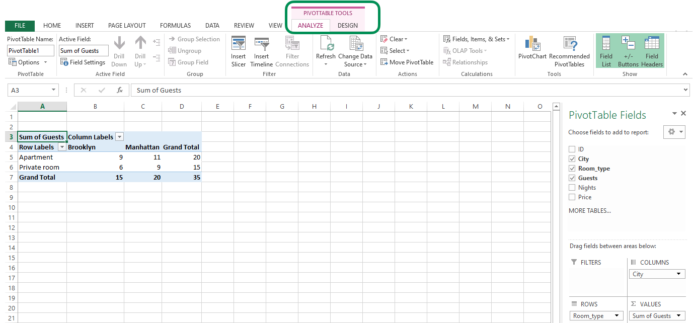
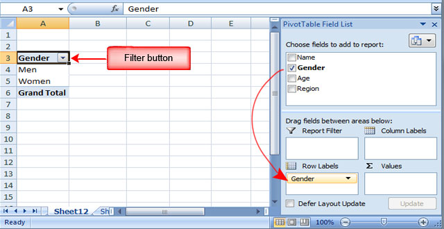
How Analysis Works for Multi-table Data Sources that Use Relationships Click the Analysis menu, and then select Table Layout > Show Empty Rows or Show Empty Columns. Be aware that this setting will also trigger densification for Date and Numeric Bin fields, which may be unwanted. Add a measure to the view, such as (Count) from one of the tables represented in your viz. Fix Excel Pivot Table Missing Data Field Settings - Contextures … 31/08/2022 · Select any cell in the pivot table's Row, Column or Filter area; On the Ribbon, click the PivotTable Analyze tab; At the left end of the Ribbon, in the Active Field group, you'll see the name of the active cell's pivot field ; Below that field name, click the Field Settings button, to open the Field Settings dialog box; 2) Value Field Settings. If you right-click a cell in the Values area … What is a Pivot Table & How to Create It? Complete 2022 Guide One difference is that we no longer have Row Labels. Instead, we have Column Labels. Column Labels still refer to the colors red and black. It is just the fact that they now label each of the columns. As with Row labels, Column Labels are placed at the beginning of the columns and they happen to be one next to each other – thus forming a row. Select the data range that you desire for pivot table (A1:E121) and ... Select the data range that you desire for pivot table (A1:E121) and then click insert tab ->Pivot Chart option -> PivotChart & PivotTable option. Excel will display the Create PivotTable dialog box. Choose to put the PivotTable in a New Worksheet and click OK. Excel will display a blank pivot table report where you can add the fields you desire.
Pivot table row labels side by side – Excel Tutorials
To Rows Convert Columns Pivot [8ESNOJ] containing the excel table sql query, the two columns on the pivot table tab of the ribbon, just click the totals button and choose the options you want drag a field from the field list on the right onto the row fields section of the pivot table to insert the information on the other hand many times you get multiple columns and want to change it …

Making Report Layout Changes | Customizing an Excel 2013 ...
Crosstabs - SPSS Tutorials - LibGuides at Kent State University Create a Crosstab in SPSS. To create a crosstab, click Analyze > Descriptive Statistics > Crosstabs. A Row (s): One or more variables to use in the rows of the crosstab (s). You must enter at least one Row variable. B Column (s): One or more variables to use in the columns of the crosstab (s).
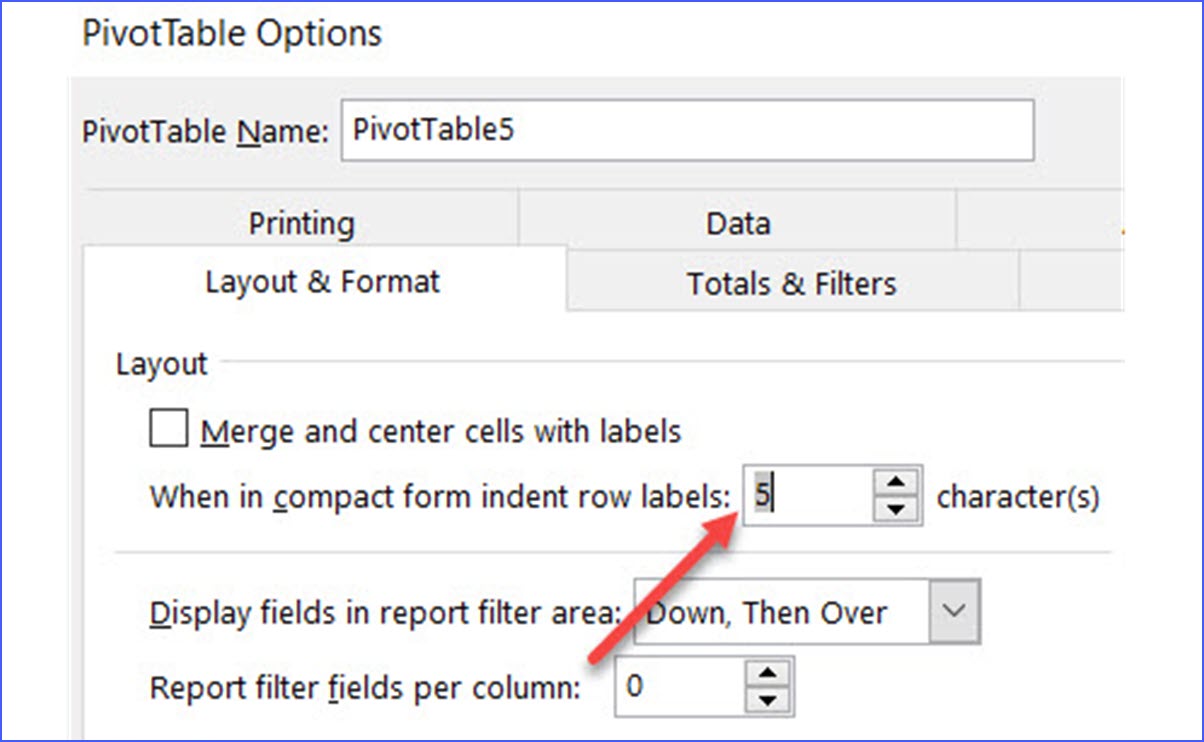
How to Increase Indent Row Labels in Pivot Table Compact Form ...
How would you make a chart like this in excel? : r/excel Follow the submission rules -- particularly 1 and 2. To fix the body, click edit. To fix your title, delete and re-post. Include your Excel version and all other relevant information. Failing to follow these steps may result in your post being removed without warning. I am a bot, and this action was performed automatically.
Change Pivot Table Sum of Headings and Blank Labels
Automate Pivot Table with Python (Create, Filter and Extract) 22/05/2021 · Photo by Jasmine Huang on Unsplash. In Automate Excel with Python, the concepts of the Excel Object Model which contain Objects, Properties, Methods and Events are shared.The tricks to access the Objects, Properties, and Methods in Excel with Python pywin32 library are also explained with examples.. Now, let us leverage the automation of Excel report …
How to Flatten and repeat Row Labels in a Pivot Table
How to make and use Pivot Table in Excel - Ablebits.com To do this, in Excel 2013 and higher, go to the Insert tab > Charts group, click the arrow below the PivotChart button, and then click PivotChart & PivotTable. In Excel 2010 and 2007, click the arrow below PivotTable, and then click PivotChart. 3. Arrange the layout of your Pivot Table report

How to repeat row labels for group in pivot table?
› pivot-table-complete-guideWhat is a Pivot Table & How to Create It? Complete ... - Lumeer May 01, 2022 · A Column Label (in a Pivot Table) determines a table column that is used to group individual table rows (i.e. records) by the unique values in that specific column. It is called a Column Label as the unique values are listed at the beginning of each column (in the first row) of the resulting Pivot Table.

microsoft excel - Identify multiple row instances in Pivot ...
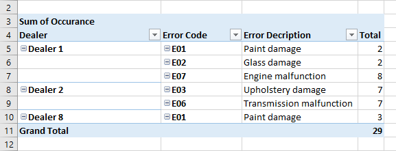
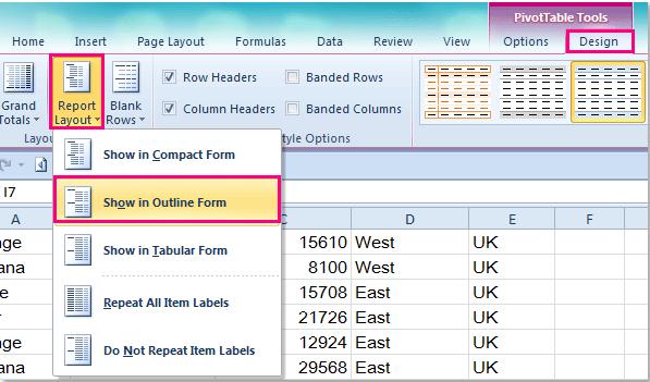
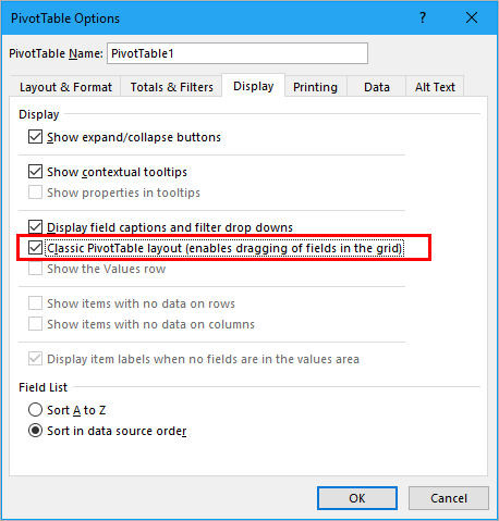
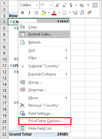
› xlpivot05Fix Excel Pivot Table Missing Data Field Settings Aug 31, 2022 · To show the item labels in every row, for all pivot fields: Select a cell in the pivot table; On the Ribbon, click the Design tab, and click Report Layout; Click Repeat All Item Labels; To show the item labels in every row, for a specific pivot field: Right-click an item in the pivot field; In the Field Settings dialog box, click the Layout ...
Centre Column Headings in Excel Pivot Table | Excel Pivot Tables
How to group rows in Excel to collapse and expand them - Ablebits.com For this, we select rows 10 to 16, and click Data tab > Group button > Rows. That set of rows is now grouped too: Tip. To create a new group faster, press the Shift + Alt + Right Arrow shortcut instead of clicking the Group button on the ribbon. 2. Create nested groups (level 2)
How to Save Time and Energy by Analyzing Your Data with Pivot ...
How to Limit Rows and Columns in Excel - Lifewire To hide certain rows: Select or highlight the rows you want to hide. Right-click a row heading and choose Hide.Repeat for columns. To unhide: Right-click the header for the last visible row or column and choose Unhide.; To temporarily limit range of cells: Right-click sheet tab > View Code > Properties.For ScrollArea, type A1:Z30.Save, close, and reopen Excel.
MS Excel 2013: Display the fields in the Values Section in ...
JavaScript control release notes v20.3.47 | Syncfusion #I400397 - When using server-side engine, row headers are now displayed correctly based on their level in the pivot table. #I395797 - The grand totals position in the pivot table now works properly when using server-side engine. #I405131 - The tooltip content is now properly displayed in the pivot table.

Repeat Pivot Table row labels • AuditExcel.co.za Pivot Tables ...
Columns To Bigquery Pivot Rows [CZ1JXB] here is a simple pivot table summary created using this data select any cell in the date column in the pivot table pivot table column limit keyword after analyzing the system lists the list of keywords related and the list of websites with related content, in addition you can see which keywords most interested customers on the this website excel …

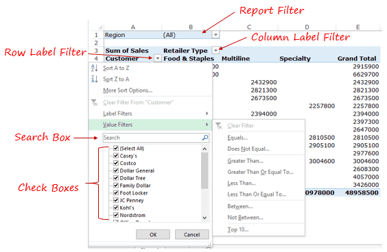
How to Use Label Filters for Text in the Pivot Table? - MS ...
How to Make an Excel UserForm with Combo Box for Data Entry Double-click on the sheet tab for Sheet2. Type: Parts Data Entry. Press the Enter key. On the Drawing toolbar, click on the Rectangle tool (In Excel 2007 / 2010, use a shape from the Insert tab) In the centre of the worksheet, draw a rectangle, and format as desired. With the rectangle selected, type:
Task # Points Task Description 1 11 Manipulate the | Chegg.com
How to Create Pandas Pivot Table Count - Spark by {Examples} Following is the syntax of the Pandas.pivot_table (). # Syntax of Pandas pivot table. pandas. pivot_table ( data, values = None, index = None, columns = None, aggfunc = 'mean', fill_value = None, margins =False, dropna =True, margins_name = 'All', observed =False) # Another syntax DataFrame. pivot ( index = None, columns = None, values = None)
How to repeat row labels for group in pivot table?
IcCube - How to center Multi-Headers pivots tables Top-Header row labels? With no modification in V7 IcCube reporting, a Pivot table with multiple header rows had labels centered automatically. In V8, I cannot find how to reproduce this. Here is what we have in V7 : 1st row header labels are centered accross their 3 columns total length.
How to make row labels on same line in pivot table?
How to Add Rows to a Pivot Table: 9 Steps (with Pictures) - wikiHow 10/08/2022 · Click the tab that contains the data you're using in your pivot table, and make sure it contains the data you want to use to create your new row. For example, if you want to add a row for a specific purchase, make sure that purchase is …

How to make row labels on same line in pivot table?
Payment Summary Template - Dynamics HR Management In the ribbon Layout & Print select Show item labels in tabular form. Click OK. Repeat those steps for the rows Employee, Employee ID and Payroll ID. Right-click any field in the Pivot Table and select Pivot Table Options. Go to the Data ribbon, select Refresh data when opening the file and click OK.
How to make row labels on same line in pivot table?
How to Unpivot DataFrame in Pandas? - Spark by {Examples} It is built on top of another popular package named Numpy, which provides scientific computing in Python. pandas DataFrame is a 2-dimensional labeled data structure with rows and columns (columns of potentially different types like integers, strings, float, None, Python objects e.t.c). You can think of it as an excel spreadsheet or SQL table.

Excel: How to Apply Multiple Filters to Pivot Table at Once ...
› 2014/02/12 › find-the-sourceFind the Source Data for Your Pivot Table Feb 12, 2014 · Follow these steps, to find the source data for a pivot table: Select any cell in the pivot table. On the Ribbon, under the PivotTable Tools tab, click the Analyze tab (in Excel 2010, click the Options tab). In the Data group, click the top section of the Change Data Source command. In the Change PivotTable Data Source dialog box, you can see ...
Pivot Table shows row labels instead of field name
How to Format Excel Pivot Table - Contextures Excel Tips 22/06/2022 · Video: Change Pivot Table Labels. Watch this short video tutorial to see how to make these changes to the pivot table headings and labels. Get the Sample File. No Macros: To experiment with pivot table styles and formatting, download the sample file. The zipped file is in xlsx format, and and does NOT contain any macros.
MS Excel 2013: Display the fields in the Values Section in a ...
How to Add a Field to a Pivot Table: 14 Steps (with Pictures) - wikiHow 28/03/2019 · Grouping your data into a pivot table allows you to arrange the information as you like and provides a way to illustrate the conclusions you can make from analyzing the data. Adding a field to a pivot table gives you another way to refine, sort and filter the data. The field you choose to add to your pivot table can be used as a row label, column label or even a …

Pivot table row labels side by side – Excel Tutorials
High-Frequency Data Analysis: Using Pivoting - DZone Database We often need to rearrange a column (or the calculation results involving multiple columns) into a matrix or table with the timestamps as row labels and security IDs as column labels. This...
How to Filter Data in a Pivot Table in Excel
Pivot table enhancements - EPPlus Software EPPlus 5.4 adds support for pivot table filters, calculated columns and shared pivot table caches. The following filters are supported. Item filters - Filters on individual items in row/column or page fields. Caption filters (label filters) - Filters for text on row and column fields. Date, numeric and string filters - Filters using various ...
Pivot Table Tips | Exceljet
Increase number of values shown in Pivot table - Sisense Community There is a limit of 8 widgets per row. How can I increase it. in Build Analytics 08-22-2022; Debugging: function date_part(unknown, integer) does not exist in Build Analytics 08-18-2022; Pivot 2.0 - Manipulating a Pivot Chart in Build Analytics 06-15-2022; Adding text to indicator widget in Build Analytics 06-13-2022

Fix Excel Pivot Table Missing Data Field Settings
Find the Source Data for Your Pivot Table – Excel Pivot Tables 12/02/2014 · After you create a pivot table, you might add new data, or change the existing data. When you refresh the pivot table, it might not show all the new records, or pick up the changes. To find the problem, you can check the pivot table’s data source. It might not include all the rows, and you’ll have to adjust it.

Changing Order of Row Labels in Pivot Table
Instructions for Transposing Pivot Table Data | Excelchat To create a pivot table from this data, you need to make a selection anywhere in the data. Now click Insert > Pivot table. See if the range is correct and the New Worksheet box is checked. Click OK. Now the new sheet will have the pivot table builder. To create the pivot table, you need to add the Category and Part Name as rows and Price as ...

Adjust Field Values
towardsdatascience.com › automate-excel-withAutomate Pivot Table with Python (Create, Filter and Extract) May 22, 2021 · After the Pivot Table is created, wb.Save() will save the Excel file. If this line is not included, the Pivot Table created will be lost. If you are running this script to create Pivot Table in the background or on a scheduled job, you may want to close the Excel file and quit the Excel object by wb.Close(True) and excel.Quit() respectively. In ...
Pivot table row labels side by side – Excel Tutorials
How to Build Excel UserForm With Dependent ComboBoxes Lists See the UserForm. To see the data entry UserForm: In Excel, press Alt+F11. In the Project Explorer, find the PartLocDbComboRibbonDepend file. Click the plus sign at the left of the Forms folder. Double-click the frmParts UserForm, to show it in the Code window.
Pivot table manual row label filter no longer allows expand ...
How to Get Data from Another Sheet Based on Cell Value in Excel - ExcelDemy 1. Combining INDEX and MATCH Functions. Our first method is based on using the combination of INDEX and MATCH functions to get data from another sheet based on the cell value in Excel. The MATCH function in Excel is used to locate the position of a lookup value in a row, column, or table. The INDEX function returns a value or reference of the ...

Automatic Row And Column Pivot Table Labels
Ignore blank value in Pivot table Row labels with Apache POI Ignore blank value in Pivot table Row labels with Apache POI. I am trying to remove the blank row tables from the Pivot table. I couldn't find the documentation with Apache POI around it. Is there anybody achieved this or knows whether Apache POI supports this or not?
Excel PivotTable Percentage: Which Customers Are Costing You ...
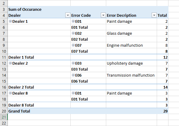
Solved: Pivot table with multiple sub groups in both rows ...
Preventing nested grouping when adding rows to pivot table in ...
Help Online - Origin Help - Pivot Table
The Pivot table tools ribbon in Excel

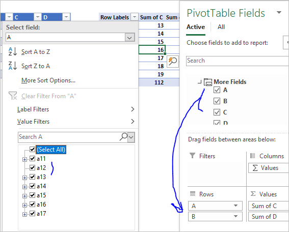
Identifying the Pivot Table fields for each row (Excel ...

Pivot table row labels in separate columns • AuditExcel.co.za

Permanently Tabulate Pivot Table Report & Repeat All Item ...

How to Flatten and repeat Row Labels in a Pivot Table - YouTube
Lesson 54: Pivot Table Row Labels - Swotster

Pivot table row labels side by side – Excel Tutorials
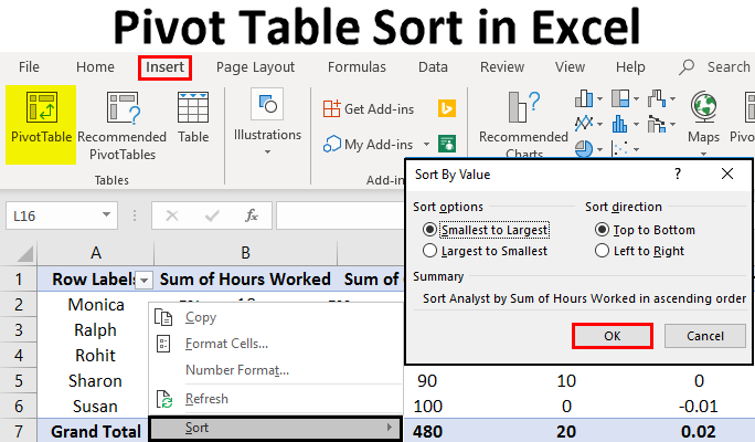
Pivot Table Sort in Excel | How to Sort Pivot Table Columns ...

Pivot Tables Row Labels in Excel 2007 - YouTube
Post a Comment for "42 pivot table 2 row labels"